How Vimeo stores Video Content Ratings at Scale
Howdy!
Today we’ll be talking about
The Engineering behind Canva’s Analytics Platform
Canva is a web application that you can use to make graphics. They offer a Pro version as a monthly subscription.
They overhauled their data analytics infrastructure and that’s given them much more flexibility.
Lessons learned from the overhaul
How Vimeo stores Video Content Ratings at Scale
Vimeo is a video sharing platform with over 100 million videos uploaded yearly. Some of these videos contain nudity, explicit language, etc. which users may want to filter out.
Engineers encode video content ratings and user filters as bit fields that are stored in integers, resulting in huge time/space efficiencies compared to using a hash table or array.
We’ll talk about how it works
Plus, some tech snippets on
How to create good looking websites while sucking at design
Monarch: Google’s planet-scale in-memory Time Series Database
Creating an open source version of OpenAI’s DALL-E 2
We have an answer to our last question on sorting the elements in a stack. We also have a new question from Bloomberg.
The Engineering Behind Canva’s Analytics Platform
Canva is a web application that you can use to make graphics (logos, charts, social media banners, etc.). The company has more than 60 million monthly active users and does more than $1 billion in annual revenue.
Their main revenue source is Canva Pro, a monthly subscription product that users can upgrade to for additional features (background remover, more animations/fonts, etc.).
Chuxin Huang and Paul Tune are two machine learning engineers at Canva, and they wrote a great blog post about the architecture of the analytics stack they use for optimizing Canva to maximize revenue.
Here’s a summary
Canva Pro offers a monthly or yearly subscription. Users start with a 14 day free trial.
The pro service was first launched in 2015 and built on Stripe’s subscription service. They used third party services (Profitwell) to keep track of annual recurring revenue, conversion rates, churn, etc. This setup allowed the company to launch the product quickly and see how it was received by users.
As Canva scaled, the company needed to build a better data stack so they could get more detailed metrics and data. They wanted the ability to drill down into specific customer segments (based on country, monthly/yearly plan, etc.) and analyze metrics by group. Additionally, Canva’s subscription model has some differences compared to a standard subscription model, so Profitwell’s metrics weren’t entirely accurate.
When designing the new data platform, the team optimized for the following
Scalability - In the future, Canva will add new subscription plans, pricing options, etc. The data model should easily scale accordingly.
Flexibility - Analysts should be able to easily split up the data based on customer demographics and create metrics based on new business needs.
Trustworthy - Data quality and accuracy is essential as the reports generated from the data platform will be used for product/management decisions and also given to investors.
Accessibility - The data platform should be accessible to all of Canva’s internal teams: product, growth, finance, design, engineering, etc.
New Data Platform
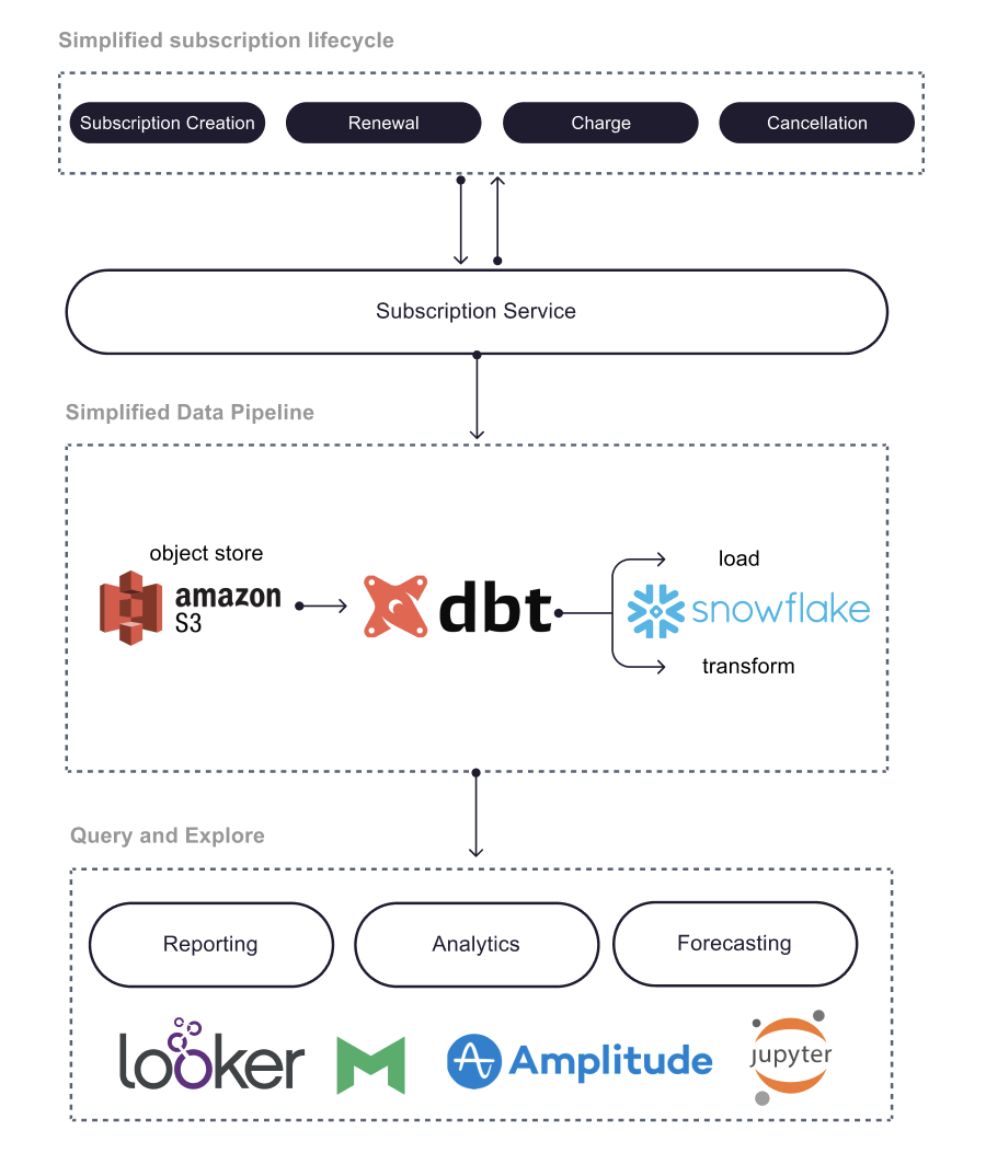
Here’s the architecture of Canva’s new platform for subscription data.
With this architecture, they’ve gotten big improvements from two factors.
First, the Data team redesigned the schema of Canva’s core subscription database tables.
They linked and aggregated information from multiple sources on things like subscription creation, billing data, user profile data (geography, usage, etc.), attribution and more. This makes it much easier for analysts to quickly gather all the relevant information they need to make a report.
Second, the change in the tooling of the platform made a big difference. They migrated to Snowflake (a data warehouse) and use Snowflake SQL.
They also found Data Build Tool (dbt) to be extremely useful for templating and sharing functions for data transforms.
The data pipeline is doing a process called ETL (Extract, Transform, Load), where you first
Extract all the necessary data from all your different sources (third party companies like Stripe, different services in your backend, etc.)
Transform the data (cleaning) by striping out what you don’t want, reformatting it, testing for inaccuracies, etc.
Load the data into your data warehouse (Snowflake in this case).
dbt is a command line tool that data analysts can use for the transform part of ETL and it makes it much easier to apply software engineering practices (version control, code review, automated testing, etc.) to the data transformation functions being written for data cleaning.
At the end of the stack, data analysts and business users can use tools like Looker, Mode and Amplitude for data visualization and reporting.
Data scientists and machine learning engineers can use Jupyter for building prediction models.
Results
The new pipeline made it much easier to measure metrics like churn, customer lifetime-value, conversion rates, etc.
The article goes into detail on exactly how Canva measures churn (they use a statistical model called the Fader-Hardie model) so you should definitely check out the full blog post if you’re interested in that.
Machine learning engineers at the company are also developing models based on the new data infrastructure. One of the applications is a predictor (based on logistic regression) that estimates the probability that a customer converts from a trial to becoming a paid user.
Lessons Learned
An important lesson that Canva learned was to be sure to invest in proper data infrastructure and analytics before applying machine learning. Your ML models are only as good as the data that goes into them.
For data analytics, it’s essential to first have a solid data infrastructure with reliable processes for data collection, ingestion and quality checks. The underlying infrastructure should also perform fast, reliably and efficiently at scale.
For more details, you can read the full post here.
Tech Snippets
Monarch: Google’s Planet-Scale In-Memory Time Series Database - Micah Lerner is a software engineer at Google and he writes a great blog where he goes over interesting papers on computer science. In this post, he goes over Monarch, Google’s system for storing time series metrics.
LAION-5B dataset - You’ve probably seen some of the amazing images produced by OpenAI’s DALL-E 2. However, the dataset that OpenAI used to create the model (and the source code) was not released publicly.
LAION-5B is an awesome effort to build an open, free dataset of over 5 billion image-text pairs so that anyone can recreate DALL-E 2 (and answer many more fascinating research questions).
Yannic did a great interview with the leaders of the project to talk about their motivations, goals and the engineering behind the effort.
How to create great looking websites while sucking at design - If you’ve ever tried to build a website, you’ll quickly realize how difficult it is to make something that looks nice. This is a great blog post with some advice on how you can make websites that look visually appealing while having the artistic sense of a donkey.
How Vimeo stores Video Content Ratings at Scale
Vimeo is a video sharing platform with more than 200 million users and over 100 million videos uploaded yearly.
Users on the platform can select content filters for things they want to avoid, like nudity, explicit language, violence, etc.
In order to keep track of these content filters in an efficient way, Vimeo uses bit manipulation. Radhika Kshirsagar is a software engineer at Vimeo, and she wrote a great blog post on the engineering they use.
Here’s a summary
Vimeo has a variety of different content filters that they need to keep track of; things like nudity, violence, drugs, explicit language, etc.
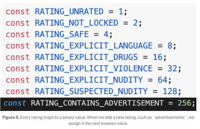
They keep track of these using a bit field data structure, where each bit represents a specific content filter flag (nudity, violence, etc.). If the video is unrated, then the 0th bit will be set to 1. If the video contains explicit language, then the 3rd bit will be set to 1.
The entire bit field can fit in a single integer, so comparing bit fields can be done in O(1) - constant time. This makes it incredibly memory and time efficient.
Every user on the Vimeo platform will also have their own bit field that keeps track of their viewing preferences. If a user is okay with watching videos with nudity, then that corresponding nudity bit will be set to 1. If they flag nudity as something they want to avoid, then that bit will be set to 0.
Then, when Vimeo wants to check if a user can watch a video, the backend just has to do a bitwise AND operation between the video’s bit field and the user’s bit field.
All the 1s in the user’s bit field represent filters that the user is okay with watching, so the AND operation between the video’s bit field and the user’s bit field should result in 1s for all the matching 1 bits and 0s for all the mismatching bits or matching 0 bits.
Therefore, the result of the AND operation between the user’s bit field and the video’s bit field will be equal to the video’s bit field if the user has allowed all the content filters that the video is flagged for.
If the result of the AND operation is not equal to the video’s bit field, then that means the user has filters set to avoid the video.
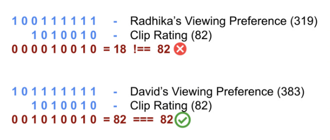
In the example above, the video clip’s bit field is 1010010, or 82 in base 10. Radhika and David are two Vimeo users who have their own viewing preferences encoded in bit fields.
Running the AND operation between Radhika’s bit field and the video’s bit field will indicate that the video clip has a 1 set in a bit where Radhika has a 0 set, so Vimeo can filter out that video for Radhika.
David has 1s set for all the fields where the video clip has a 1, so he’s eligible to watch the video.
This AND operation can be done in constant time, so it’s far quicker than having a hashmap or array keep track of a content ratings and doing an O(n) comparison every time you need to check if a user can watch the video.
For more details, you can read the full blog post here.
Interview Question
You are given an array of intervals where intervals[i] = [start_i, end_i].
Merge all overlapping intervals, and return an array of the non-overlapping intervals that cover all the intervals in the input.
Example
Input - intervals = [[1,3],[2,6],[8,10],[15,18]]
Output - [[1,6],[8,10],[15,18]]
Here’s the question in LeetCode.
Previous Question
As a refresher, here’s the previous question
Write a function that sorts the elements in a stack so that the smallest elements are on top.
You can use an additional temporary stack, but you cannot copy the elements into any other data structure.
The stack supports the following operations
push
pop
peek
isEmpty
Solution
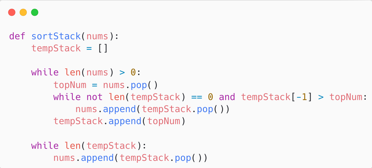
We can solve this question with a modified version of insertion sort.
In insertion sort, you build the final sorted array one item at a time, where you remove an item from the input data and find its location in the sorted list and insert it there.
For us, we’ll have our input stack and then a temporary stack (tempStack).
We’ll continuously pop off the top element from our input stack and put it in a temporary variable (topNum). We’ll then find the correct place in tempStack to insert topNum in. Our loop invariant is that tempStack will always be correctly sorted.
However, tempStack… is a stack (obviously). So, we can’t randomly insert topNum anywhere in the stack. We can only push our element to tempStack.
Therefore, rather than doing random insertions, we’ll pop elements off tempStack and append them to our input stack if the item at the top of tempStack is greater than topNum (the item we’re trying to insert in tempStack).
On the next iteration of our loop, that element becomes our new topNum and will be placed back into tempStack in it’s correct location.
We can terminate the loop when our input stack is empty.
Then, we’ll just pop and append all the elements in tempStack to our input stack.
Here’s some of our past tech dives
An introduction to Compilers and LLVM
LLVM is an insanely cool set of low-level technologies (assemblers, compilers, debuggers) that are language-agnostic. They’re used for C, C++, Ruby, C#, Scala, Swift, Haskell, and a ton of other languages.
This post goes through an introduction to compiler design, the motivations behind LLVM, the design of LLVM and some extremely useful features that LLVM provides. We’ll be giving a summary below.
Back in 2000, open source programming language implementations (interpreters and compilers) were designed as special purpose tools and were monolithic executables. It would’ve been difficult to reuse the parser from a static compiler to do static analysis or refactoring.
Additionally, programming language implementations usually provided either a traditional static compiler or a runtime compiler in the form of an interpreter or JIT compiler.
It was very uncommon to see a language implementation that had supported both, and if there was then there was very little sharing of code.
The LLVM project changes this.
Introduction to Classical Compiler Design
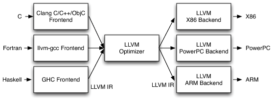
The most popular design for traditional static compilers is the three-phase design where the major components are the front end, the optimizer, and the back end.
Front End
The front end parses the source code (checking it for errors) and builds a language-specific Abstract Syntax Tree.
The AST is optionally converted to a new representation for optimization (this may be a common code representation, where the code is the same regardless of the input source code’s language).
Optimizer
The optimizer runs a series of optimizing transformations to the code to improve the code’s running time, memory footprint, storage size, etc.
This is more or less independent of the input source code language and the target language
Back End
The back end maps the optimized code onto the target instruction set.
It’s responsible for generating good code that takes advantage of the specific features of the supported architecture.
Common parts of the back end include instruction selection, register allocation, and instruction scheduling.
The most important part of this design is that a compiler can be easily adapted to support multiple source languages or target architectures.
Porting the compiler to support a new source language means you have to implement a compiler front end for that source language, but you can reuse the optimizer and back end.
The same applies for adding a new target architecture for the compiler. You just have to implement the back end and you can reuse the front end and optimizer.
Additionally, you can use specific parts of the compiler for other purposes. For example, pieces of the compiler front end could be used for documentation generation and static analysis tools.
The main issue was that this model was rarely realized in practice. If you looked at the open source language implementations prior to LLVM, you’d see that implementations of Perl, Python, Ruby, Java, etc. shared no code.
While projects like GHC and FreeBASIC were designed to compile to multiple different CPUs, their implementations were specific to the one source language they supported (Haskell for GHC).
Compilers like GCC suffered from layering problems and leaky abstractions. The back end in GCC uses front end ASTs to generate debug info and the front end generates back end data structures.
The LLVM project sought to fix this.
LLVM’s Implementation of the Three-Phase Design
In an LLVM-based compiler, the front end is responsible for parsing, validating, and diagnosing errors in the input code.
The front end then translates the parsed code into LLVM IR (LLVM Intermediate Representation).
The LLVM IR is a complete code representation. It is well specified and is the only interface to the optimizer.
This means that if you want to write a front end for LLVM, all you need to know is what LLVM IR is, how it works, and what invariants it expects.
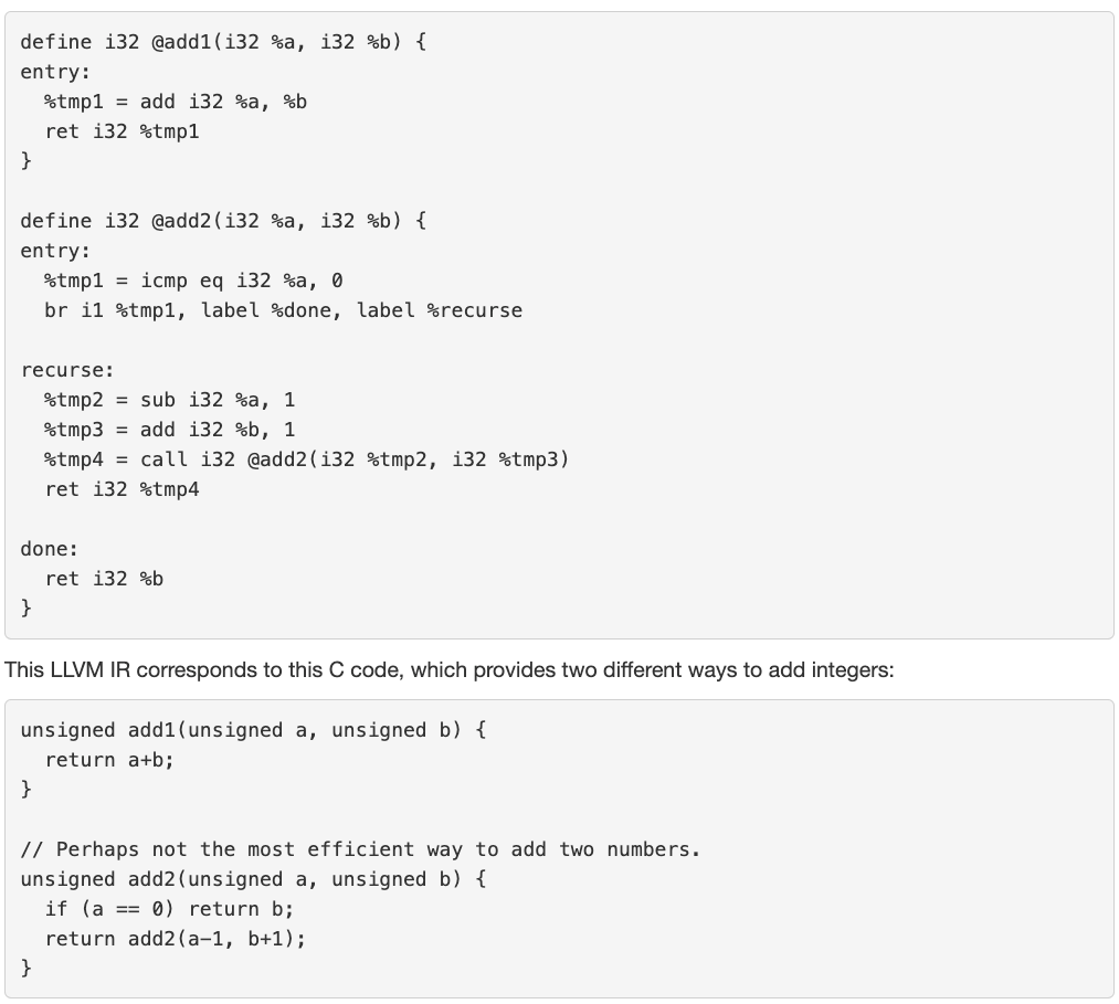
LLVM IR is a low-level RISC-like virtual instruction set and it is how the code is represented in the optimizer. It generally looks like a weird form of assembly language.
Here’s an example of LLVM IR and the corresponding C code.
Now, the optimizer stage of the compiler takes the LLVM IR and optimizes that code.
Most optimizations follow a simple three-part structure:
Look for a pattern to be transformed
Verify that the transformation is safe/correct for the matched instance
Do the transformation, updating the LLVM IR code
An example of an optimization is pattern matching on basic math expressions like replacing X - X with 0 or (X*2)-X with X.
You can easily customize the optimizer to add your own optimizing transformations.
After the LLVM IR code is optimized, it goes to the back end of the compiler (also known as the code generator).
The LLVM code generator transforms the LLVM IR into target specific machine code.
The code generator’s job is to produce the best possible machine code for any given target.
LLVM’s code generator splits the code generation problem into individual passes- instruction selection, register allocation, scheduling, code layout optimization, assembly emission, and more.
You can customize the back end and choose among the default passes (or override them) and add your own target-specific passes.
This allows target authors to choose what makes sense for their architecture and also permits a large amount of code reuse across different target back ends (code from a pass for one target back end can be reused by another target back end).
The code generator will output target specific machine code that you can now run on your computer.
For a more detailed overview and details on unit testing, modular design and future directions of LLVM, read the full post!
A browsable Petascale Reconstruction of the Human Cortex
A connectome is a map of all the neural connections in an organism’s brain. It’s useful for understanding the organization of neural interactions inside the brain.
Releasing a full mapping of all the neurons and synapses in a brain is incredibly complicated, and in January 2020, Google Research released a “hemibrain” connectome of a fruit fly - an online database with the structure and synaptic connectivity of roughly half the brain of a fruit fly.
The connectome for the fruit fly has completely transformed neuroscience, with Larry Abbott, a theoretical neuroscientist at Columbia, saying “the field can now be divided into two epochs: B.C. and A.C. — Before Connectome and After Connectome”.
You can read more about the fruit fly connectome’s influence here.
Google Research is now releasing the H01 dataset, a 1.4 petabyte (a petabyte is 1024 terabytes) rendering of a small sample of human brain tissue.
The sample covers one cubic millimeter of human brain tissue, and it includes tens of thousands of reconstructed neurons, millions of neuron fragments and 130 million annotated synapses.
The initial brain imaging generated 225 million individual 2D images. The Google AI team then computationally stitched and aligned that data to produce a single 3D volume.
Google did this using a recurrent convolutional neural network. You can read more about how this is done here.
You can view the results of H01 (the imaging data and the 3D model) here.
The 3D visualization tool linked above was written with WebGL and is completely open source. You can view the source code here.
H01 is a petabyte-scale dataset, but is only one-millionth the volume of an entire human brain. THe next challenge is a synapse-level brain mapping for an entire mouse brain (500x bigger than H01) but serious technical challenges still remain.
One challenge is data storage - a mouse brain could generate an exabyte of data so Google AI is working on image compression techniques for Connectomics with negligible loss of accuracy for the reconstruction.
Another challenge is that the imaging process (collecting images of the slices of the mouse brain) is not perfect. There is image noise that has to be dealt with.
Google AI solved the imaging noise by imaging the same piece of tissue in both a “fast” acquisition regime (leading to higher amounts of noise) and a “slow” acquisition regime (leading to low amounts of noise). Then, they trained a neural network infer the “slow” scans from the “fast” scans, and can now use that neural network as part of the connectomics process.


